A deep dive into Transformer models like GPT and BERT (English version)
To provide the theoretical basis for understanding models such as GPT and BERT, I outline some concepts of the Transformer architecture in this blog post. To do this, I discuss feedforward neural networks in 1. In section 2, I describe recurrent neural networks with an encoder-decoder architecture and the first attention mechanism. In 3, I bring all the elements together to describe a Transformer model. Finally, in 4, I discuss some specifics of GPT models and BERT.
This article has two aims. On the one hand, Transformer models are to be explained via their historical genesis, which is why I recommend reading sections 1 and 2, whereby the focus here should be on the processing of sequences with an encoder-decoder structure. Secondly, the Transformer models are based on a ‘new’ (i.e. new for 2017) self-attention mechanism, which is also worth understanding mathematically. Once again, it will hopefully not be difficult for readers to understand this once they have an intuition for previous attention mechanisms. This blog entry is intended as an aid to understanding the Transformer model. Nevertheless, I recommend that you also read the publications cited. It makes sense to read them in chronological order.
1 Feedforward neural networks
1.1 Definition of a neural network
In abstract terms, a neural network is initially an approach for approximating a function \(f(X; \theta)\) that can be used to map the input values \(X\) with the parameters \(\theta\) (Goodfellow et al. 2016). For example, as a classifier, a network with the correct parameters would predict \(f(x)=y\), where \(y\) corresponds to a class label (Goodfellow et al. 2016).
Neural networks consist of a number of linked functions that process an input to an output using a directed circle-free graph. The respective functions can also be referred to as layers \(h_{i}\) with \(i \in N\) and \(N\) as the corresponding depth of the network. The last layer is called the output layer \(a\) (cf. Fig. 1). Instead of considering each function of a layer as a mapping of a vector to a vector, the functions should rather be understood as compositions of units that together map vectors to scalars that together will form a new vector (Goodfellow et al. 2016).
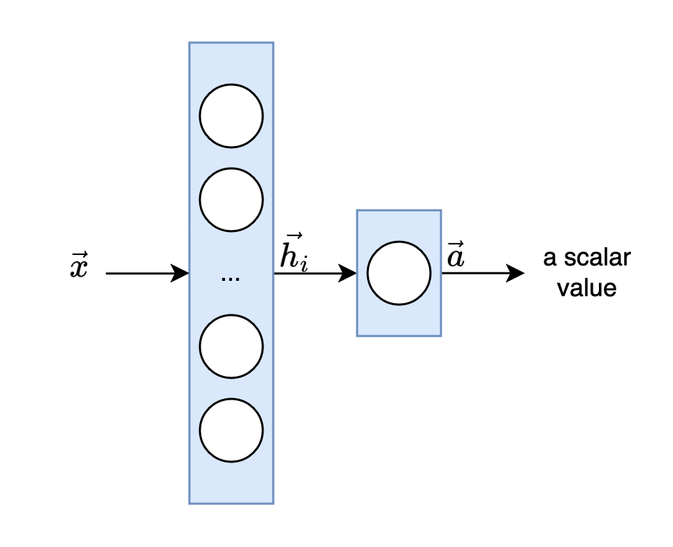
Fig. 1: A neural network with input \(x\), layer \(h_i\), and output layer \(a\)
The set of linked functions of a neural network also includes non-linear functions (activation functions). We can define the layers as follows: \begin{equation} h_{linear} := W \cdot x + b \end{equation} \begin{equation} h_{non-linear} := \sigma(W \cdot x + b) \end{equation} where \(W\) is a matrix with weights, \(x\) the input, \(b\) additional biases, and \(\sigma\) an activation function (e.g., sigmoid, tanh, softmax). A neural network is described as feedforward if no form of feedback is taken into account from the input to the output of the information flow (Goodfellow et al. 2016).
1.2 Training of a neural network
The approximation of the parameters \(\theta\) (i.e. the weights and biases of the network) follows the typical machine learning scheme of three steps for each training instance.
- For \(x \in X\) the network predicts a value \(y\).
- This value is ‘evaluated’ with another function, a loss function (also often called an objective function). The losses provide information on the extent to which the prediction of the network differs from a target value (typical loss functions are e.g. Mean Squared Error or Cross Entropy). By including a target value (sometimes also referred to as ground truth), this can also be referred to as supervised learning. We’ll see that training a language model on text is a form of self-supervised learning.
- To reduce future losses, an optimization algorithm adjusts all parameters of the network based on the loss function. The goal is to minimize the loss by approximating its global (or at least a good local) minimum. The influence of each parameter on the loss is determined through its gradient, which is computed using the chain rule across the entire network. By leveraging these gradients, the model updates its parameters in a way that reduces the loss over subsequent predictions.
2 Recurrent neural networks with an encoder-decoder architecture
2.1 Definition of a recurrent neural network
In contrast to feedforward networks, recurrent neural networks exchange information within a layer with the states \(h_{i}^{t}\) (also called hidden states). Each state at time \(t\) not only receives information from the input, but also from previous inputs, such as \(x_{t-1}\), and their states, i.e. from \(h_{i}^{t-1}\) and so on (cf. Fig. 2).
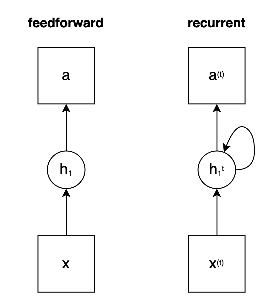
Fig. 2: Status of a neural network without (feedforward) and with feedback (recurrent) and in each case an input layer \(x\), a hidden layer \(h_1\) and an output \(a\)
The advantage of recurrent neural networks such as the Long Short-Term Memory Model (LSTM for short in Hochreiter and Schmidhuber, 1997) is that they are particularly good at modelling sequential data such as speech. A net should base its prediction for an input from a sentence also on previous words. As inspired by Ferdinand de Saussure: The meaning of a word is derived from the interplay of the differences of the surrounding words (de Saussure, 1931). Thus, even a neural network can derive little meaning from an isolated consideration of each word. However, if the meanings of the surrounding word inputs are included in a layer of a recurrent network, i.e. a sequence as a whole, more information is taken into account.
2.2 Auto-regressive language models (LMs)
With these tools, we can already develop a simple language model (LM) for predicting sequences. Suppose we want a model that generates a sequence \(w\) with \(w=(w_{1}, w_{2}, w_{3}, ..., w_{n})\), where \(n\) corresponds to the length of the words belonging to the sequence, for example a sentence. A much-used approach in natural language processing is to derive the prediction of each word from all previous words in the sequence. We can illustrate this idea with the chain rule for probabilities as follows: \begin{equation} p(w) = p(w_{1}) \cdot p(w_{2}|w_{1}) \cdot p(w_{3}|w_{1}, w_{2}) \cdot … \cdot p(w_{n}|w_{1}, …, w_{n-1}) \end{equation} At this point, it is already useful to understand that we are following an auto-regressive prediction of the sequence, where each word is treated as dependent on all previous words.
Applied to machine learning using the data \(w\), it follows from the proposed language modelling that we want to approximate the following function: \begin{equation} p(w; \theta) \end{equation} i.e. we are looking for the best parameters \(\theta\) with language data (also called corpora) for our model, with which we can achieve a prediction for a sequence of words \(w\) that corresponds to the data used. We can realise the approximation by training both a simple feedforward neural network and a recurrent one. The recurrent neural network has the advantage that it better incorporates the preceding words by passing additional information through the states within each of its layers.
2.3 Encoder-decoder models for machine translation (MT)
Using LSTMs, Sutskever et al. (2014) develop a sequence-to-sequence architecture for machine translation (MT). Their approach combines two important ideas. Firstly, a translation should be conditioned by the original language, i.e. a translated sentence \(O\) (output) depends on its original sentence \(I\) (input). Secondly, translations cannot always be carried out literally. For this reason, it makes sense for a model to consider the whole original sentence before predicting a potential translation.
The first idea (a) leads to the conditional language models: \begin{equation} p(w | c; \theta) \end{equation} In these models, the prediction of the word sequence not only depends on each preceding word, but is also conditioned by the source sentence \(c\), which is so important for the translation. In principle, however, it can also be other information that would be included in the prediction.
The second idea is implemented by Sutskever et al. (2014) by developing an architecture consisting of two parts, an encoder and a decoder (see Fig. 3) (see also Cho et al. 2014). Whereby the encoder summarizes the source sentence into a fixed representation \(c\) and then passes it to the decoder to predict the translation in the target language.
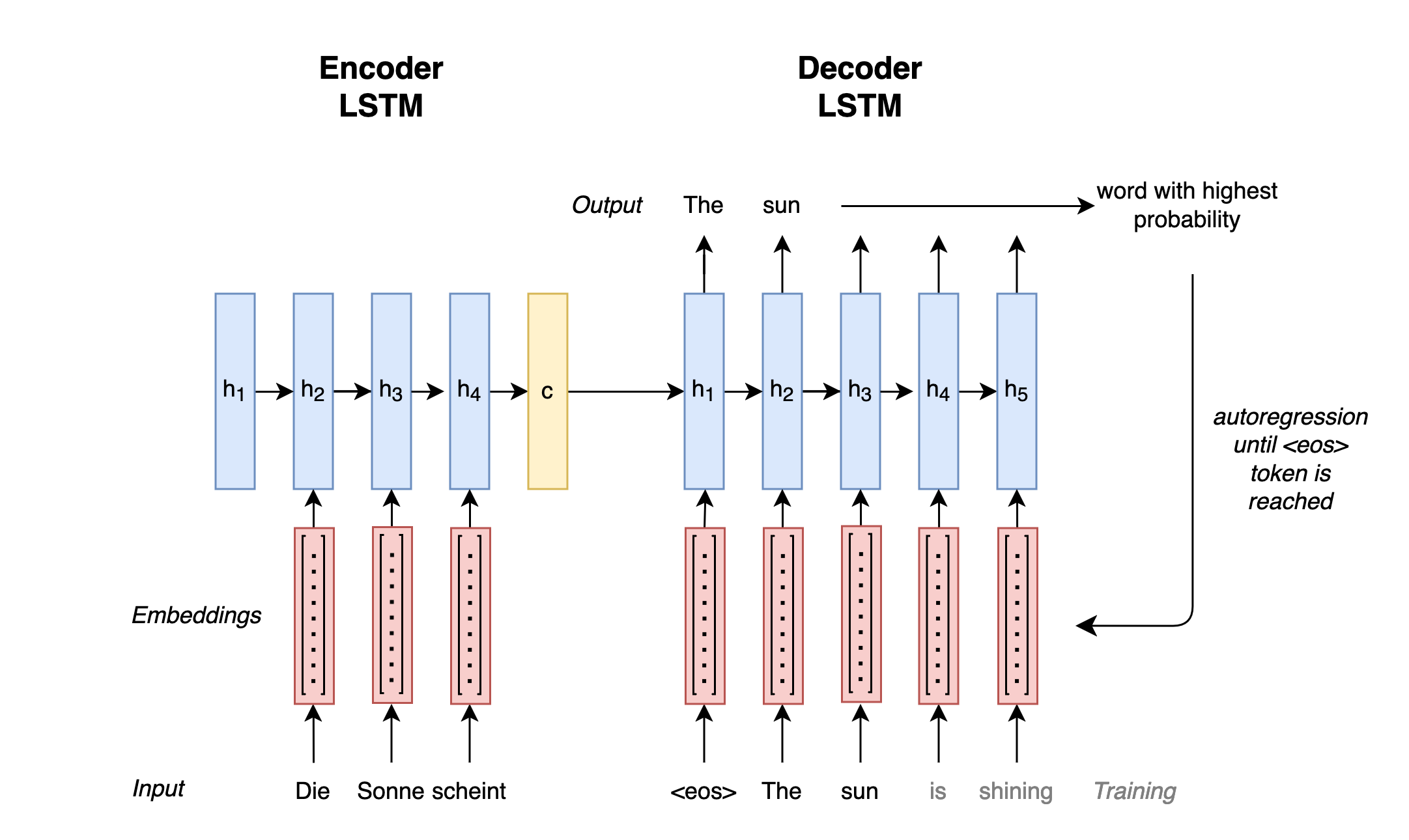
Fig. 3: Sequence-to-sequence architecture with encoder and decoder
For the encoder, Sutskever et al. (2014) use an LSTM model that is fed vector representations (also called embeddings) for the words of an input sequence from the original language. Embeddings are used for the simple reason that neural networks can only operate with numbers and not letters. The hidden states of these inputs are then merged by the model into a final state \(c\): \begin{equation} c = q({h^{1},…,h^{T}}) \end{equation} where \(q\) corresponds to the LSTM model and \(T\) to the length of the input sequence. The state \(c\) is passed to the decoder.
The decoder also consists of an LSTM model, which predicts a translation in the target language word by word based on the input state. Each translated word and the final encoder state of the original input \(c\) are regressively fed to the decoder until the model completes the translation: \begin{equation} p(w)= \prod_{t=1}^{T}p(w_{t}|{w_{1},…,w_{t-1}},c) \end{equation} It completes the translation as soon as it predicts the token <eos>. We use this special token to show the model where sequences begin and end during training. In its predictions, the model will therefore also predict this token at the end of a sequence in the best case and thus terminate the inference process itself.
Finally, one more word about the training of a sequence-to-sequence model: during training, the encoder of the model is shown sentences from the original language and its decoder is shown their translations according to a hyperparameter (e.g. with Professor Forcing (Goyal et al., 2016)), whereby the weights \(\theta\) of the encoder as well as the decoder can always be learned together and matched to each other. This training can be again achieved with a loss function like Cross Entropy and optimization based on gradients.
2.4 The first attention mechanism
To improve the quality of translations, especially for long sequences, Bahdanau et al. (2014) introduce an attention mechanism. The weakness of Sutskever et al.’s (2014) architecture is that the input to be translated is forced into a single representation \(c\), with which the decoder must find a translation. However, not all words in a sentence play an equally important role in a translation and the relationship between the words can also vary. Whether the article in ‘the annoying man’ for ‘l’homme ennuyeux’ is translated as ‘le’ or ‘l´’, for example, depends in French on whether the article is followed by a vowel, possibly with a silent ‘h’ in front of it (Bahdanau et al. 2014). Bahdanau et al. (2014) therefore develop a mechanism that does better justice to these nuances (cf. Fig. 4).
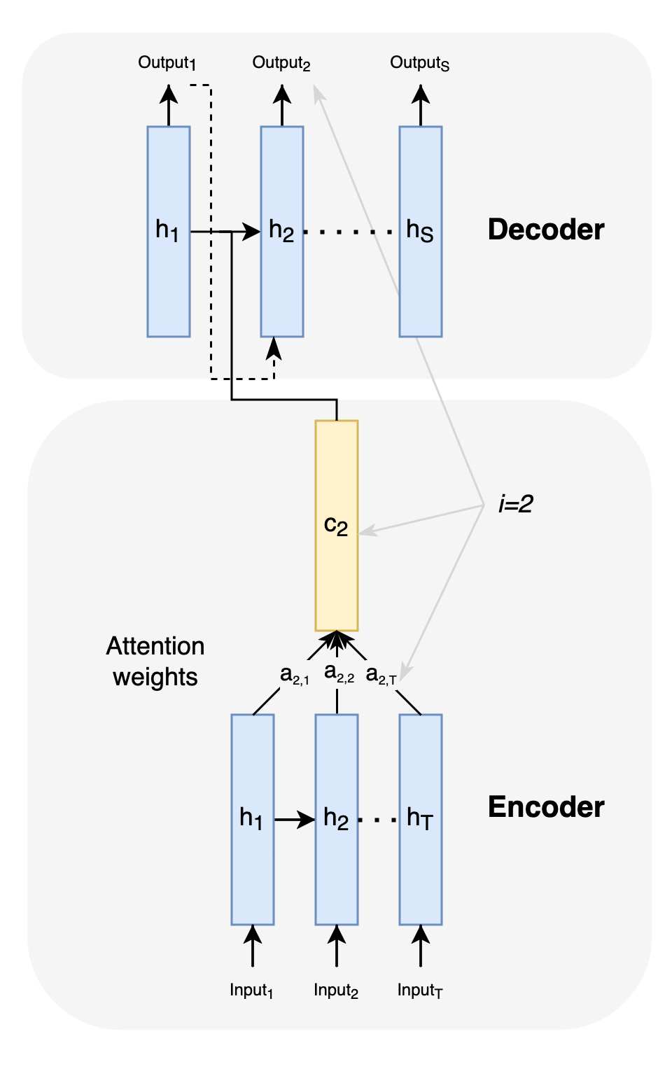
Fig. 4: Attention weights for an input with reference to the output at position i=2
The architecture extended by attention transmits context-dependent states \(c_{i}\) to the decoder instead of \(c\) for each input: \begin{equation} c_{i} = \sum_{t=1}^{T}a_{it}h^{t} \end{equation} The weight \(a_{it}\) for each state \(h^{t}\) (also called ‘annotation’ in (Bahdanau et al. 2014)) is determined as follows: \begin{equation} a_{it} = \frac{\exp(e_{it})}{\sum_{k=1}^{T}\exp(e_{ik})} \end{equation} where \(a_{it}\) is a normalization (softmax function) for the model \(e_{it}\). This model is again a feedforward network with a single layer that evaluates how well the input at time \(t\) matches the output at position \(i\). Thus, overall, each input \(x^{1}...x^{T}\) receives its own set of attention weights, resulting in \(c_{i}\), a context vector that helps the decoder determine the appropriate output (e.g. ‘l’homme’) for each input.
3 Transformer models with self attention
3.1 The structure of a Transformer model
The Transformer architecture (Vaswani et al., 2017) combines some of the previously mentioned elements. The architecture gives the attention mechanism a much greater role and dispenses with recurrent structures.
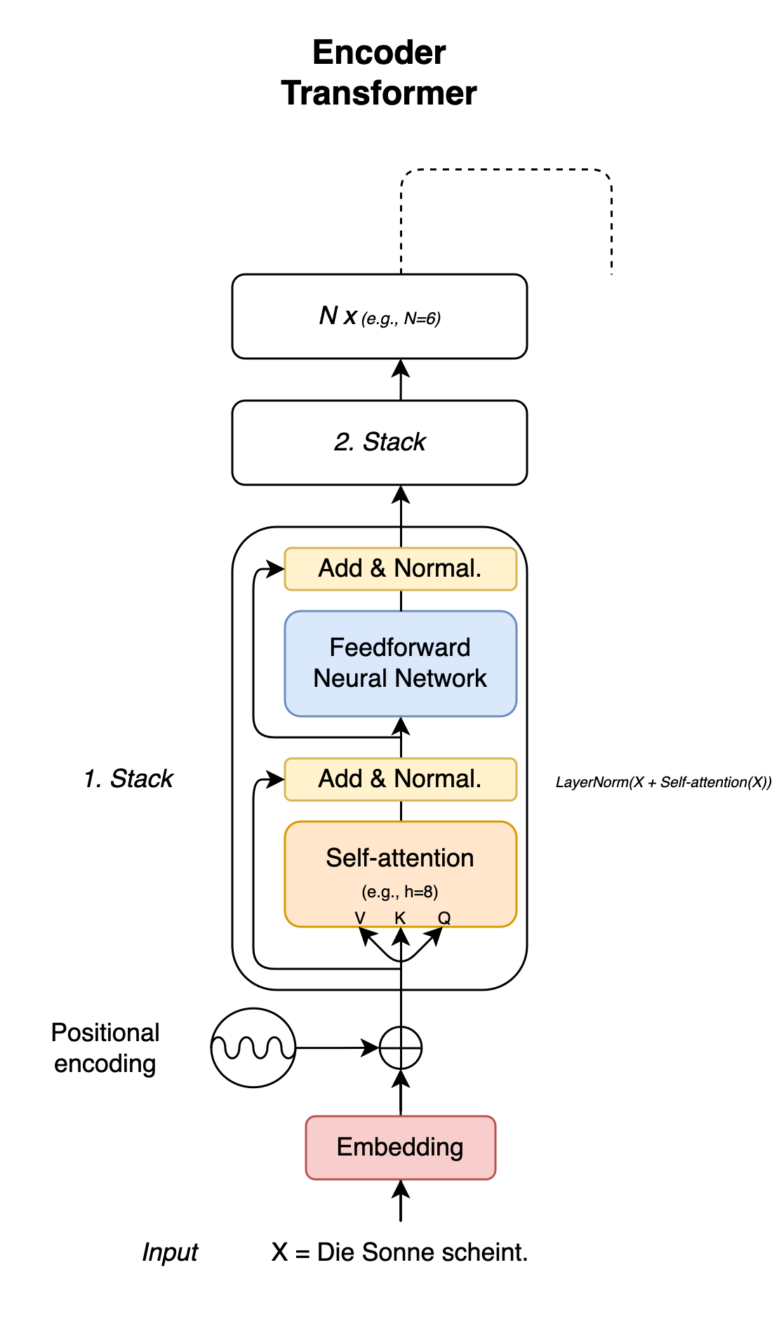
Fig. 5: Encoder of a Transformer model
The encoder of the Transformer architecture consists of stacks, each with two components, through which the incoming information is processed (see Fig. 5). Inputs are first fed in parallel to a layer with a self-attention mechanism, which is presented in Vaswani et al. (2017). After this mechanism has been applied, the information is normalized and then passed to another layer with a feedforward neural network. With this network, the processing of the input takes place individually. With an intermediate normalization step, mean values and standard deviations are calculated according to the principle of layer normalization (Ba et al. 2016; there is also root square layer normalization by Zhang & Sennrich (2019), which was used in Llama 2, for example). In addition, the normalized output is added to the output of the previous layer. This is also referred to as ‘residual connection’ and is a method to counteract the problem of disappearing gradients during backpropagation.
3.2 Embeddings with positional encoding
As with the previous sequence-to-sequence architectures, the input is first converted into embeddings. However, the embeddings are additionally provided with positional encoding, which is realized via a frequency representation (sine and cosine functions). The reason for this is as follows. In contrast to the recurrent approaches, the attention layer of a Transformer encoder processes an input sequence all at once and not word by word in the case of a translation, for example. Without additional information on the position of each input within a sequence, the coders would lack the important information on how the individual words follow each other.
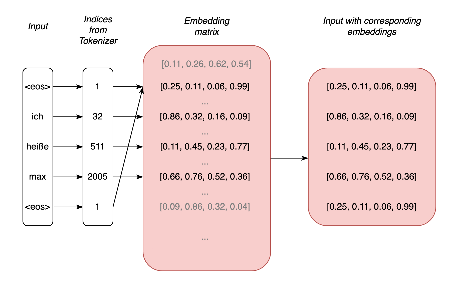
Fig. 6: Example sequence whose tokens are converted into embeddings with \(d=4\)
For processing the input, the Transformer architecture provides an embedding matrix for all vocabulary of the data that is used in the training of a Transformer model. The size of the matrix corresponds to the number of vocabulary words (otherwise referred to as tokens, which also include punctuation marks, for example) with a selected dimension (i.e. n x d), with which each input token can be assigned exactly one row within the matrix (cf. Fig. 6). The number of columns corresponds to the selected dimension. The matrix values for the token types are randomly selected during the initialization of a Transformer model. It is the rows of this matrix that are also referred to as embeddings. It can also be said that each token type has a vector representation. In a further step, these vectors are added to the positional encoding to give the input a unique representation. It is crucial that the embeddings of the Transformer architecture also change in the course of training, i.e. they can be adapted according to the data, i.e. ‘learned’. (Note 1: the first step is to convert the input tokens into an index representation based on a tokenizer, with which each token can be assigned a row in the embedding matrix; note 2 – and this took me some time to understand: BERT embeddings and the like are not those embeddings from the input; these embeddings are rather the result of the attention mechanisms and extracted from the end of a Transformer layer).
To illustrate positional encoding, it is helpful to first consider a very simplified example. Assume that each embedding is simply assigned the positions (pos) of the respective token in the form of integers with \(n \in N\), where \(N\) corresponds to the length of the input tokens including <eos> tokens. If we select the token “heiße” and its embedding [0.11, 0.45, 0.23, 0.77] (imaginary values), then a positional encoding of [2, 2, 2, 2] could be determined for the token within the sequence “<eos> ich heiße max <eos>” as follows. The vector of the token would have these values because we chose the second position of the sequence (sequence starts at 0) and an embedding dimension of \(d=4\). According to the Transformer architecture, we could then add this vector to the embedding of the token [2.11, 2.45, 2.23, 2.77] and thus add additional information to it. However, this approach would lead to several problems; for example: large position values for long sequences would override the values of the embeddings and a relative reference of recurring positional patterns would be missing.
Vaswani et al. (2017, p. 6) therefore present positional encodings that provide each token embedding with additional information about the position of the token within a sequence via the radians of the trigonometric functions. The advantages of this approach include the fact that the positional encoding values can be limited to an interval of \([-1,1]\), and the periodicity of the trigonometric functions also allows recurring patterns to be mapped. This is so because certain distances between positions will produce similar values. This makes it easier for the model to learn that certain patterns or distances between tokens are repeated in different areas of a sequence, regardless of the exact position in the sequence.
According to Vaswani et al. (2017), the positions of the tokens are calculated as follows: \begin{equation} PE_{(pos, 2i)} = sin(\frac{pos}{10000^{\frac{2i}{d}}}) \end{equation} \begin{equation} PE_{(pos, 2i+1)} = cos(\frac{pos}{10000^{\frac{2i}{d}}}) \end{equation} pos corresponds to the absolute position within an input sequence of length N, the value \(10000\) is a selected constant, and i refers to the indices of the embeddings. For example, for a selected dimension of the embedding vectors with \(d=4\), \(i \in I= \{0, 1, 2, 3\}\) applies. Finally, the two sine and cosine functions allow different values to be determined for even and odd indices. We can use (10) for all even indices of an embedding and (11) for all odd indices. It is worth mentioning here that the frequencies of the sine and cosine functions of the PE depend on the selected dimension. Small ebedding dimensions lead to higher frequencies (finer position resolutions) and high dimensions to lower frequencies (coarser position resolutions). Based on these specifications, a positional encoding matrix is finally calculated for each input – i.e. a position vector for each token (see Fig. 7). In combination with the embeddings, the Transformer model is given a context-sensitive representation of the tokens for further processing in this fashion.
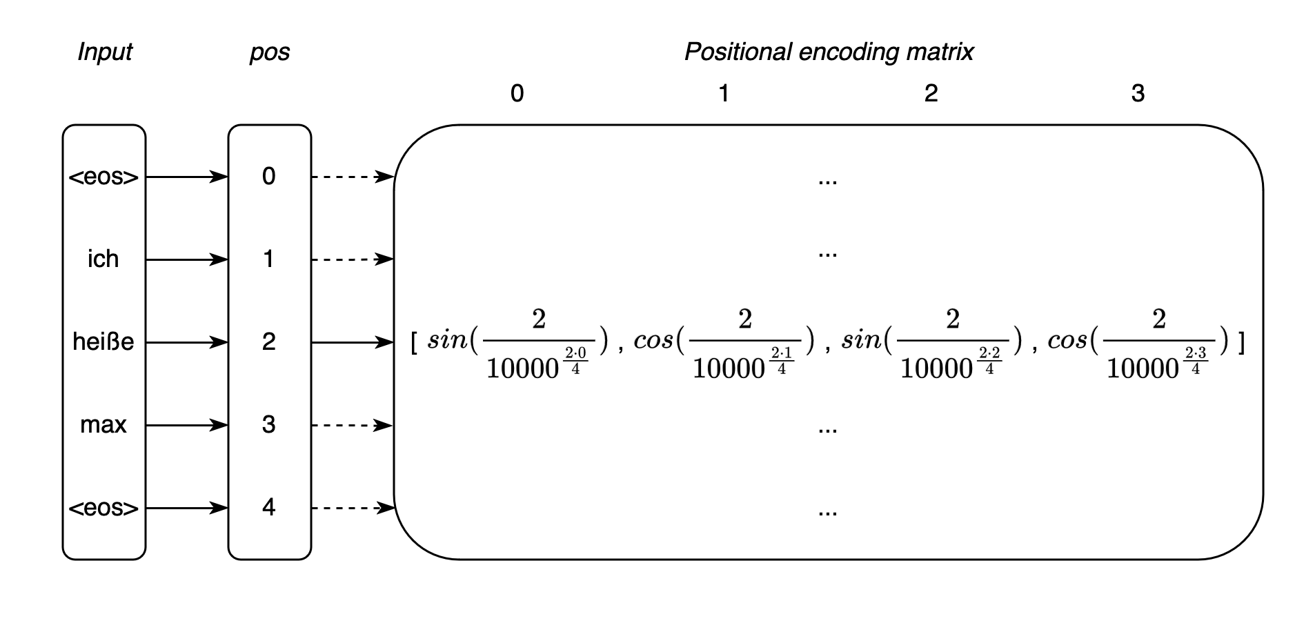
Fig. 7: Exemplary sequence, whose tokens are mapped to positional encodings with \(d=4\)
3.3 Self-attention
In contrast to the attention mechanism according to Bahdanau et al. (2014), Vaswani et al. (2017) develop a self-attention mechanism, which they also describe as ‘scaled scalar product attention’ (Vaswani et al., 2017, p.3). In simplified terms, the self-attention used for Transformers can first be compared with the operation from (8) (Raschka et al., 2022). We can calculate the attention for a context-sensitive vector \(z_{i}\) of an input at position \(i\) as follows (Raschka et al., 2022): \begin{equation} z_{i} = \sum_{j=1}^{T}a_{ij}x^{j} \end{equation} where \(a_{ij}\) is not multiplied by a state \(h^{t}\), but by the inputs \(x^{j}\), with \(j\in{\{1, ..., T\}}\) an input sequence of length \(T\) (cf. the sum over all \(x^{j}\) in (12)). In contrast to Bahdanau et al. (2014), \(a\) is not a normalization of simple feedforward networks \(e_{ij}\), but a softmax normalization over the scalar products \(\Omega\) of the input \(x^{i}\) related to all other inputs \(X=x^{1}, ..., x^{T}\) (Raschka et al., 2022): \begin{equation} a_{ij} = \frac{\exp(\omega_{ij})}{\sum_{j=1}^{T}\exp(\omega_{ij})} \end{equation} with (Raschka et al., 2022): \begin{equation} \omega_{ij} = x^{(i)T}x^{j} \end{equation} What we also see here, in contrast to the attention mechanism of Bahdanau et al. (2014), in which attention includes in particular the output of the decoder (there at output position i), is that the attention weight in (13) with (14) refers to the other inputs of a sequence. For this very reason, it makes sense to speak of self-attention.
To this representation of attention, Vaswani et al. (2017) add a further change for each input \(x^{i}\), namely the weight \(a\) is not multiplied by \(x^{j}\), but by a value \(v^{j}\): \begin{equation} z_{i} = \sum_{j=1}^{T}a_{ij}v^{j} \end{equation} Vaswani et al. (2017) transform each \(x^{i}\) into a triple of (\(v^{i}\), \(k^{i}\), \(q^{i}\)) using the projection matrices (\(W_{v}\), \(W_{k}\), \(W_{q}\) – which can also be understood here as additional linear layers). The idea behind this comes from information retrieval, which works with value, key and query triples (hence the abbreviations v, k, q). The V, K, Q in Fig. 5 and Fig. 10 correspond to: \(V=XW_{v}\), \(K=XW_{k}\) and \(Q=XW_{q}\) (cf. Fig. 9). The scalar products of the self-attention mechanism for each input are also not calculated with (14) in Vaswani et al. (2017), but with the query and key values (Raschka et al., 2022): \begin{equation} \omega_{ij} = q^{(i)T}k^{j} \end{equation} Finally, the attention weights are scaled with the dimension of the embeddings (\(\frac{\omega_{ij}}{\sqrt{d}}\)). Vaswani et al. (2017, p. 4) justify the additional scaling with the observation that too large values of the scalar products (see (14)) lead the softmax function used for additional normalization into a range that results in very small gradients during learning.
In short: In addition to the attention of an input \(x^i\) to all other inputs within a sequence \(X\), the self-attention is calculated by different representations of all \(x^j \in X\) in the form of query, key and value representations. Self-attention can be also described as a scoring mechanism that determines the relevance of neighboring tokens for each token (consider Fig. 8).
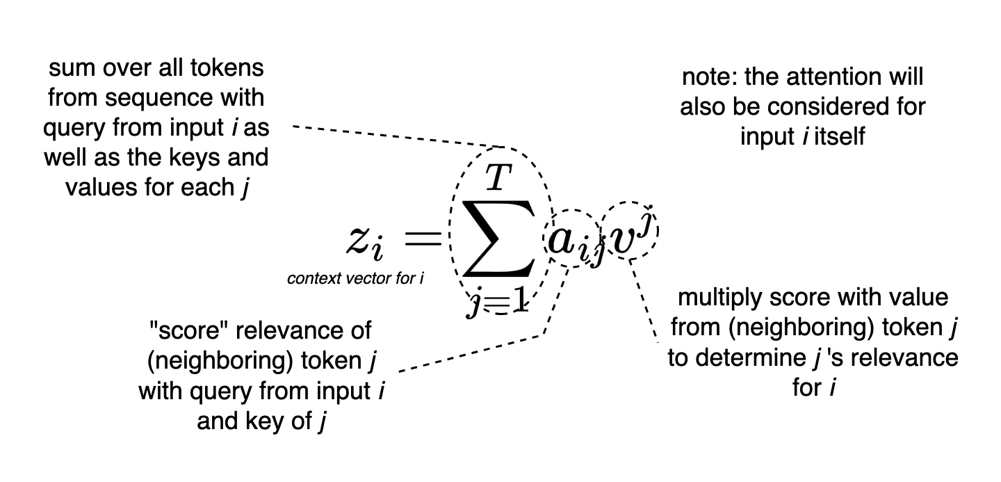
Fig. 8: Attention mechanism as a score to determine relevance of tokens from context
Attention can be calculated \(h\) times in parallel, where \(h\) corresponds to a selected number of heads (also called attention heads). Vaswani et al. (2017) choose \(h=8\) heads, whose values are concatenated and finally passed on to the layer normalization in the coders (see Fig. 9 and Fig. 5). The use of multiple heads is referred to as ‘multi-head attention’.
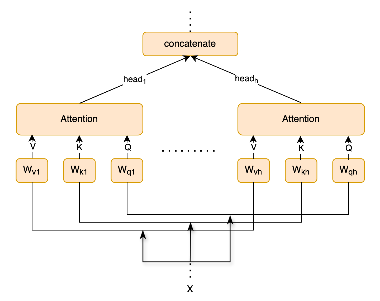
Fig. 9: Attention for input \(X\) with multiple heads
3.4 The Transformer decoder
The decoder of the Transformer architecture follows the structure of the encoder. However, it contains an additional layer (see Fig. 10). In this layer, the information output by the encoder (e.g. the encoded original sentence of a translation) is also taken into account via the value and key values \(V\), \(K\). The query values \(Q\), on the other hand, come from the previous attention layer of the decoder. Due to the combination of information from both the encoder and the decoder, this additional layer is also referred to as the ‘cross-attention layer’. Since encoder information is included, the whole model (encoder + decoder) can also be referred to as a conditional language model, as previously presented in (5).
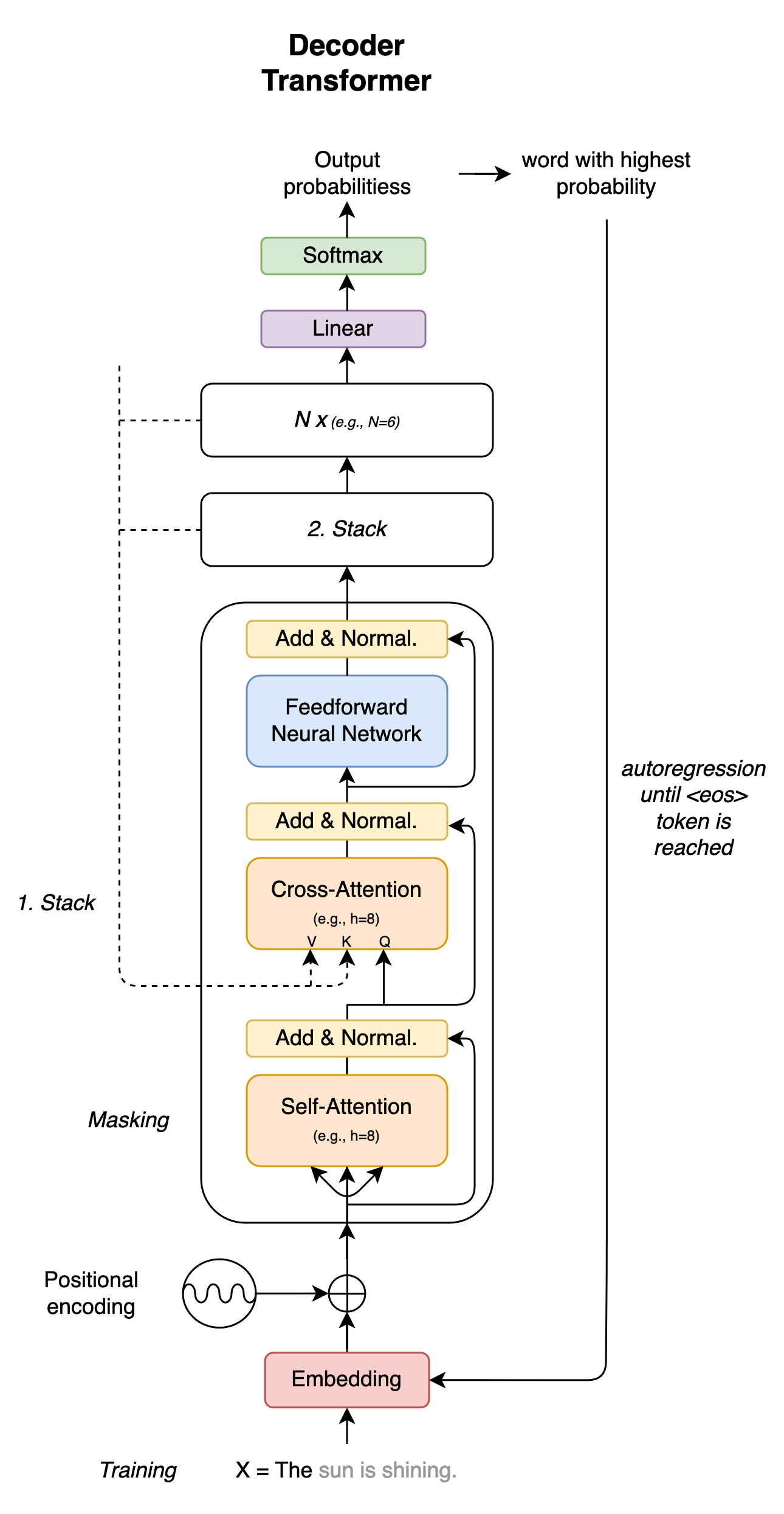
Fig. 10: Decoder of a Transformer model
The self-attention layer of the decoder allows parts of the decoder input to be masked (this is also described as masking, or more precisely causal masking). A Transformer encoder, on the other hand, allows all inputs to be viewed simultaneously. Masking plays an important role in the goal of the decoder: e.g. the prediction of a translation. To predict a translation sequence, the decoder works autoregressively from token to token (e.g. from left to right, see also (7)). This means that during inferencing, each prediction only works with the help of previous tokens, the others remain masked in a figurative sense. For training, correct translations can be added to the model as input by Professor Forcing in order to minimize error propagation – as with the sequence-to-sequence models described above. Basically, the training goal is to optimize the predictions of the model based on the translation solutions. A translation process terminates in any case when the token <eos> or the previously defined maximum sequence length is reached.
Finally, a word about the linear layer at the end of the decoder (see Fig. 10). The immediate output from the attention blocks comprises a representation of the input embeddings \(h_{i}\) enriched by the model. Additional information from surrounding tokens and the encoder has been incorporated into this representation through the attention mechanisms and the feedforward neural networks. Now each \(h_{i}\) must be converted back into a representation of the vocabulary. For this purpose, the linear layer provides a projection matrix \(W\). This is similar to a layer of a neural network with the difference that no non-linear activation function further alters the information flow.
Let’s look at an example. Suppose the model is based on a vocabulary size of \(10 000\) and we choose a dimension of \(d=512\) as an example for the embeddings or the status of the model. We can then use \(W\) (10000 x 512) to convert all \(h_{i}\) into a logits vector that corresponds to the dimension of the vocabulary and whose value is also the model’s approximation of how likely each of the vocabulary’s tokens is: \begin{equation} logits = W \cdot h_{i} + b \end{equation} where \(b\) as an additional bias has an influence on the mapping. Based on this logits vector (e.g. \(logits = [3.4, -1.2, 0.5, ..., 2.7]\)), the softmax activation, with which the values of the vector are converted into probabilities, can finally predict the most probable token for the output status \(h_{i}\) of the decoder. However, other decoding strategies (e.g. beam search or greedy decoding) could also be used at this point.
Overall, inference and training in a Transformer model do not differ from other neural networks (see chapter 1.2).
4 GPT, BERT and co
While the original Transformer architecture was developed for machine translation, Transformer models have also proven themselves in other tasks. The best known are large language models such as Generative Pre-trained Transformer models (Radford et al., 2018) from OpenAI, which ‘continue’ an input (prompt) with a Transformer decoder, i.e. predict the next tokens of the sequence. Language models such as GPT consist of only decoder stacks. The Bidirectional Encoder Representations from Transformers model (BERT for short, Devlin et al., 2019) is in turn a pure Transformer encoder. This means that BERT cannot be used to generate new words or sentences in a target language through autoregression. Instead, BERT provides encodings that can be used to solve classification tasks, for example. In general, the development of most Transformer models consists of two phases: pre-training, and fine-tuning for specific applications. Finally, I will present these two steps with BERT.
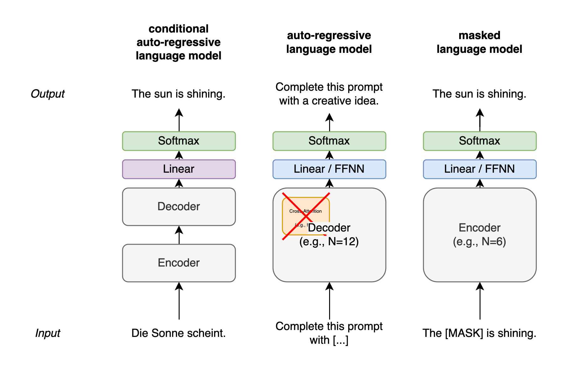
Fig. 11: Different Transformer architectures: encoder-decoders for machine translation (also called MTM), single decoders for sequence generation (also called LM), and single encoders for downstream tasks (also often called MLM)
4.1 The Bidirectional Encoder Representations from Transformers model
For BERT, Devlin et al. (2019) first train the encoder of a Transformer model against the background of two tasks. The first task of the BERT training consists of masked language modeling (MLM). The model is shown sentences in which it has to predict 15% randomly selected words that are masked. The second task consists of a binary classification of two sentences with the aim of predicting whether or not they follow each other. The model is shown 50% correct sentence sequences and 50% incorrect sequences. Since the model only uses an encoder – and no ‘right-aligned’ masking of the next tokens within a sequence is performed as with a Transformer decoder – the training can also be described as bi-directional. The encoder has access to the inputs from both sides. Devlin et al. (2019) refer to the training of their encoder on the two tasks as pre-training.
In a further step, Devlin et al. (2019) use the pre-trained BERT model for experiments in natural language processing. For example, they fine-tune BERT to classify the most plausible word sequence for sentences from the data set Situations With Adversarial Generations (Zellers et al., 2018). To do this, BERT is shown various possible continuations for training. The model must select the most plausible one from these. Since BERT was originally pre-trained against the background of other tasks, but the weights of the model can also be used and adapted for such new tasks, such fine-tuning of BERT can also be described as a form of transfer learning.
Additional resources
- I can recommend Brendan Bycroft’s visualizations of Transformer models: https://bbycroft.net/llm
- Lena Voita provides excellent explanations and visualizations of different modeling approaches in NLP, including the Transformer architecture: https://lena-voita.github.io/nlp_course.html
- Jay Alammar provides further helpful visualizations of BERT: https://jalammar.github.io/illustrated-bert/
Bibliography
Ba, J., Kiros, J.R., & Hinton, G.E. (2016). Layer Normalization. ArXiv, abs/1607.06450.
Bahdanau, D., Cho, K., und Bengio, Y. (2014). Neural Machine Translation by Jointly Learning to Align and Translate. CoRR, abs/1409.0473.
Cho, K., van Merri ̈enboer, B., Gulcehre, C., Bahdanau, D., Bougares, F., Schwenk, H., and Bengio, Y. (2014). Learning Phrase Representations using RNN Encoder–Decoder for Statistical Machine Translation. In Moschitti, A., Pang, B., and Daelemans, W., editors, Proceedings of the 2014 Conference on Empirical Methods in Natural Language Processing (EMNLP), Seiten 1724–1734, Doha, Qatar. Association for Computational Linguistics.
de Saussure, F. (1931). Cours de Linguistique Generale. Payot, Paris.
Devlin, J., Chang, M.-W., Lee, K., and Toutanova, K. (2019). BERT: Pre-training of Deep Bidirectional Transformers for Language Understanding. In Burstein, J., Doran, C., und Solorio, T., editors, Proceedings of the 2019 Conference of the North American Chapter of the Association for Computational Linguistics: Human Language Technologies, Volume 1 (Long and Short Papers), pages 4171–4186, Minneapolis, Minnesota. Association for Computational Linguistics.
Goodfellow, I., Bengio, Y., and Courville, A. (2016). Deep Learning. MIT Press.
Goyal, A., Lamb, A. M., Zhang, Y., Zhang, S., Courville, A. C., and Bengio, Y. (2016). Professor Forcing: A New Algorithm for Training Recurrent Networks. In Lee, D., Sugiyama, M., Luxburg, U., Guyon, I., und Garnett, R., Herausgeber, Advances in Neural Information Processing Systems, Band 29. Curran Associates, Inc.
Hochreiter, S. and Schmidhuber, J. (1997). Long Short-Term Memory. Neural Comput., 9(8):1735–1780.
Radford, A., Narasimhan, K., Salimans, T., and Sutskever, I. (2018). Improving Language Understanding by Generative Pre-Training. Technical report, OpenAI.
Raschka, S., Liu, Y., and Mirjalili, V. (2022). Machine Learning with PyTorch and Scikit-Learn: Develop machine learning and deep learning models with Python. Packt Publishing.
Sutskever, I., Vinyals, O., and Le, Q. V. (2014). Sequence to sequence learning with neural networks. In Proceedings of the 27th International Conference on Neural Information Processing Systems - Volume 2, NIPS’14, pages 3104–3112, Cambridge, MA, USA. MIT Press.
Vaswani, A., Shazeer, N., Parmar, N., Uszkoreit, J., Jones, L., Gomez, A. N., Kaiser, L. u., and Polosukhin, I. (2017). Attention is All you Need. In Guyon, I., Luxburg, U. V., Bengio, S., Wallach, H., Fergus, R., Vishwanathan, S., und Garnett, R., editors, Advances in Neural Information Processing Systems, Band 30. Curran Associates, Inc.
Zellers, R., Bisk, Y., Schwartz, R., and Choi, Y. (2018). SWAG: A Large-Scale Adversarial Dataset for Grounded Commonsense Inference. In Riloff, E., Chiang, D., Hockenmaier, J., und Tsujii, J., editors, Proceedings of the 2018 Conference on Empirical Methods in Natural Language Processing, pages 93–104, Brussels, Belgium. Association for Computational Linguistics.
Zhang, B., and Sennrich, R. (2019). Root mean square layer normalization. Proceedings of the 33rd International Conference on Neural Information Processing Systems. Curran Associates Inc., Red Hook, NY, USA.
Version 1.1
Enjoy Reading This Article?
Here are some more articles you might like to read next: